Determining anomalies in a Hadoop cluster event stream
Monitoring of the progress of these Hadoop jobs is critical as it servers the software that runs on top of the clusters.
Production Hadoop cluster tasks:
- Extract-Transform-Load (ETL) workloads
- SQL queries
- data stream tasks
CEP(Complex Event Processing): Hadoop system does not provide sufficient monitoring functionality by itself so we leverage logs generated by Hadoop and system metrics collected by Ganglia generated data that can be queried to monitor Hadoop job progress. The cluster logs are is a 1100+ columns(features) space with more than 40,000 rows(data points). Each row has a unique time-stamp associated with it, and values corresponding to the 1100+ columns space. The goal is to determine the top features from the 1100+ feature space that can be attributed to the faulty behaviour of the cluster.
Other uses are:
- Find tasks that cause cluster imbalance
- Find data pull stragglers
- Compute the statistics of a lifetime of mappers and reducers
Consider a scenario where we try to find the reason for the anomalous behaviour of a cluster. A cluster is a combination of disk, memory, CPU utilization, networking in addition to software like load balancers, mappers and reducers, name servers that can be the source of faulty behaviour of the cluster.
Exstream is a methodology to determine what is the origin of faulty behaviour and produce explanations. For example CPU utilization could be low due to large number of page faults. These could be due to a faulty disk at the node.
Work uses three desirable criteria for determining how well the explanations are:
- Conciseness: The system should prefer smaller and consequently more ingenuous explanations
- Consistency: The system should produce explanations that are consistent with ground-truth identified by humans.
- Prediction power: Generate explanations that have predictive power for proactive monitoring.
Let us quickly discuss why some of the more traditional approaches like supervised machine learning may either fail or simply be unsuitable for this problem, and how Exstream can overcome this limitation.
-
Logistic regression, Neural network models are not interpretable
-
Decision trees models are interpretable but they lack consistency, conciseness and contain correlated features
Main Approach Important Techniques
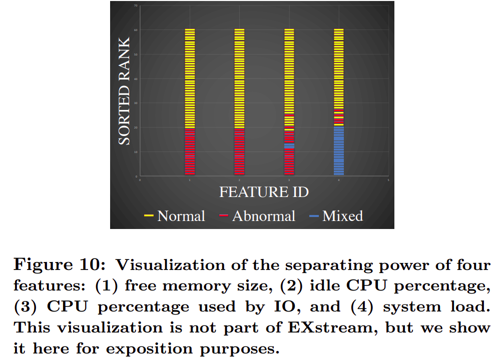
Rank the features based on a distance function. The distance function will help us know which feature is causing the anomaly. We compare the anomaly interval with a reference interval i.e the difference in the events that occur within each interval.
Use the distance function to compare the values of a feature during the 2 intervals. These features are ordered in increasing order with a value being assigned to each of them. Ranked them based on how well they separate for any given anomalous window.
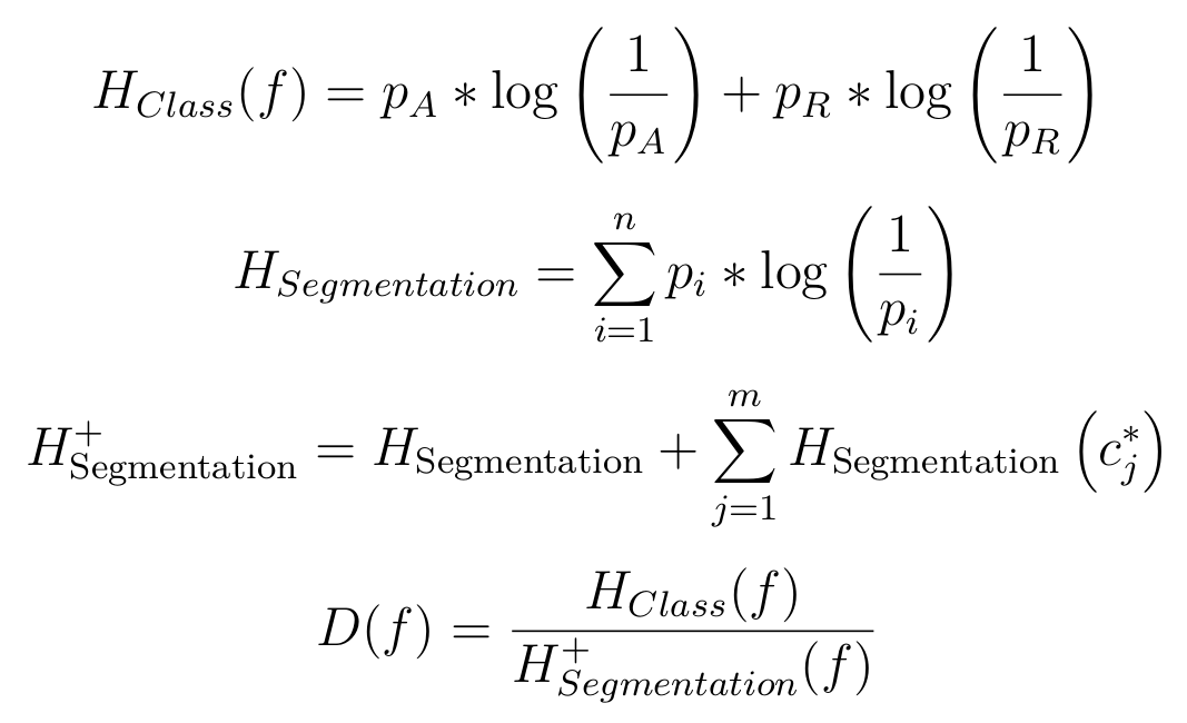
Entropy based distance function uses amount of segmentation in a feature, lets call it segmentation Entropy. Segmentation entropy is the information needed to describe how merged points are segmented by class labels.
The actual entropy being used though is the regularized segmentation entropy which is the sum of segmentation entropy and a penalty term for mixed segments.
The distance function is normalized as the features can be of different sizes. This however is not enough to construct explanations. The feature set is pruned till we get a high quality explanation. For this certain steps such as reward leap filtering, false positive filtering and filtering by correlation clustering are carried out. To build the final explanations, we need to examine the ranges of the features in the anomalous windows and generate the final explanation.
Step 0: Load the required libraries
To implement this, we use the pandas framework.
The vectorized implementations provided in pandas can allow for faster data processing which is critical to implement Exstream.
import pandas as pd
Step 1: Load the processed logs
df = pd.read_csv('preprocessed_benchmark_userclicks_11_20_10003_1000000_batch146_17_.csv')
Step 2: Clean the data
- Remove features with all same values
- Remove features with unique values
- Fill missing data with averages
import matplotlib.pylab as plt

len_dict = {}

for col in df.columns:
  len_dict[col] = len(df[col].unique())

new_dict_temp = {k: v for k, v in sorted(len_dict.items(), key=lambda item: item[1])}

plt.bar(range(len(new_dict_temp)), list(new_dict_temp.values()), align='center')
plt.xticks(range(len(new_dict_temp)), list(new_dict_temp.keys()))
plt.show()

for col in df.columns:
    if len(df[col].unique()) < 3:
        df.drop(col,inplace=True,axis=1)
df.info()
<class 'pandas.core.frame.DataFrame'>
RangeIndex: 43086 entries, 0 to 43085
Columns: 1048 entries, t to node8_VM_slabs_scanned
dtypes: float64(1033), int64(15)
memory usage: 344.5 MB
Step 3: Create ranges for anomalous and reference intervals.
The logs are in form of time-series. The range where there is a fault in the cluster is called as anomalous, the rest can be termed as reference interval.
Load anomalous and reference interval data into separate data frames.
anamlous_df = df.copy()
temp_df = df.copy()
# l = [1529015034,1528999019, 1529002179, 1529030089,1529023063,1529007602]
# l.sort()
arange1=[1528999019,1528999419]
arange2=[1529002179,1529003079]
arange3=[1529007602,1529008102]
arange4=[1529015043,1529016293]
arange5=[1529023063,1529023763]
arange6=[1529030089,1529031589]


wrange = [1528994856, 1529038088]

rrange1 = [wrange[0],arange1[0]]
rrange2 = [arange1[1]+1,arange2[0]]
rrange3 = [arange2[1]+1,arange3[0]]
rrange4 = [arange3[1]+1,arange4[0]]
rrange5 = [arange4[1]+1,arange5[0]]
rrange6 = [arange5[1]+1,arange6[0]]
rrange7 = [arange6[1]+1,wrange[1]+1]

test_list = rrange1+rrange2+rrange3+rrange4+rrange5+rrange6+rrange7
print(sorted(test_list))

an = arange1[1]-arange1[0]+arange2[1]-arange2[0]+arange3[1]-arange3[0]+arange4[1]
-arange4[0]+arange5[1]-arange5[0]+arange6[1]-arange6[0]

rf = rrange1[1]-rrange1[0]+rrange2[1]-rrange2[0]+rrange3[1]
-rrange3[0]+rrange4[1]-rrange4[0]+rrange5[1]-rrange5[0]+rrange6[1]-rrange6[0]+rrange7[1]-rrange7[0]

rr = wrange[1]-wrange[0]

print(an)
print(rf)
print(an+rf)
print(rr)
[1528994856, 1528999019, 1528999420, 1529002179, 1529003080, 1529007602, 1529008103, 1529015043, 1529016294, 1529023063, 1529023764, 1529030089, 1529031590, 1529038089]
5250
37977
43227
43232
Save the data frames as CSV files for later use
df_row_reindex.to_csv('anamlous_19.csv', index=False)
df_reference.to_csv('reference_19.csv', index=False)
#create the anamlous df
output_df = pd.DataFrame()
count = 0
for col in df_row_reindex.columns:
  count += 1
  output_df = pd.concat([output_df,df_row_reindex[col][~df_row_reindex[col].isin(df_reference[col])]], axis=1)
Step 4: Amount of Segmentation in each feature
The next task is to identify segments in each of the features. Each feature in the loaded data in the main data frame is sorted. Here, we don’t remove the repetitions as we need to account for the number of occurrences of a feature value as well. We create two new dictionaries, one contains column-wise segment type, another contains the column-wise length of each segment.
df_sorted = df.copy()

for i in df_sorted.columns:
  df_sorted[i] = sorted(df_sorted[i])
#tmp,interval_dict
from collections import defaultdict

unique_cols = tmp.keys()

dt_res = defaultdict(list)

# for col in unique_cols:
#   for i in tmp[col]:

#     if (i in reference_dict[col]) & (i in interval_dict[col]):
#       dt_res[col].append(3)

#     elif i in interval_dict[col]:
#       dt_res[col].append(1)

#     else:
#       dt_res[col].append(2)
df_res = df_sorted.copy()
for col in unique_cols:

    df_res.loc[df_sorted[col].isin(df_reference[col]), col] = 1
    df_res.loc[df_sorted[col].isin(df_row_reindex[col]), col] = 2
    df_res.loc[df_sorted[col].isin(df_reference[col]) & df_sorted[col].isin(df_row_reindex[col]), col] = 3
print(df_res['1_jvm_pools_Metaspace_committed_value'].unique())
[3. 1.]
from collections import defaultdict

dt_run = defaultdict(list)
dt_len = defaultdict(list)
for col in unique_cols:

  prev_val = None
  count = 0

  for i in df_res[col]:
    if i != prev_val:
      if count:
        dt_run[col].append(prev_val)
        dt_len[col].append(count)
      count = 1
    else:
      count += 1

    prev_val = i
  dt_run[col].append(prev_val)
  dt_len[col].append(count)
Step 5: Calulate Class Entropy
To calculate the class entropy, we count data points for anomalous and reference intervals and apply the following formula.
from math import log
entropy_dict = defaultdict()
for key,value in dt_len.items():
  s = sum(value)
  entropy = 0
  for i in range(len(value)):
    if dt_run[key][i] == 3:
      entropy += log(value[i],10)
    entropy += (value[i]/s) * log(s/value[i],10)
  entropy_dict[key] = entropy
Step 6: Calculate Segmentation Entropy
Segmentation entropy and regularization
To calculate the segmentation entropy, we use the runs and the run-lengths generated in step x. Only if we find a mixed segment, we apply the regularization penalty.
#calculation of class entropy

x,y = (df_row_reindex.shape)
a , b = df_reference.shape
# print(df_reference.shape)
# print(x)
# print(a)
# print(df.shape)
class_entropy = x/(x+a) * log((x+a)/x,10) + a/(x+a) * log((x+a)/a,10)
# print(class_entropy)
Step 7: Calculate distance by using class and segmentation entropy
#calculate distance for each feature

distance_dict = defaultdict()
for key,value in entropy_dict.items():
  if value!=0:
    distance = class_entropy/value;
    distance_dict[key] = distance
  else:
    distance_dict[key] = 0

#Remove erroneous features

dd_dict = {}
for key,val in distance_dict.items():
  if distance_dict[key] <= 1:
    dd_dict[key] = distance_dict[key]
from collections import OrderedDict
od = OrderedDict()
od = {k: v for k, v in sorted(dd_dict.items(), key=lambda item: item[1], reverse=True)}
Step 8: Leap reward filtering
In this implementation, taking the threshold for reward leap filtering by find the largest gap between any two values and removing all values below that, was leading to far less features being selected. As per the discussion in office hours, correlation-clustering is to be done before leap reward filtering, but since correlation-clustering is not required in this implementation, I devised another threshold approach based on significance. Features that are below a significance level are discarded, and only high reward features are retained. Since each workload is different, we get slightly different distance distribution, and hence different number of feature selections.
# class ExtOrderedDict(OrderedDict):
#     def first_item(self):
#         return next(iter(self.items()))

# diff_dict = {}
# prev_key,prev_value = ExtOrderedDict.first_item(od)

# print(prev_key,prev_value)
# for key,val in od.items():
#   diff_dict[key] = abs(prev_value - val)
#   #print(diff_dict[key])
#   prev_value = val
#   #print(prev_value)

# print(len(diff_dict))

# diff_dict2 = {k: v for k, v in sorted(diff_dict.items(), key=lambda item: item[1], reverse=True)}

# diff_dict3 = {}

# for key,val in diff_dict2.items():
#   if val < 0.01: ##Entropy significance level
#     break;
#   diff_dict3[key] = val
# print(diff_dict3)

# final_dict = {}

# diff_dict3 = {k: v for k, v in sorted(diff_dict3.items(), key=lambda item: item[1], reverse=False)}
# check_key,check_val = ExtOrderedDict.first_item(diff_dict3)

# for key,val in od.items():
#   if key == check_key:
#     break
#   else:
#     final_dict[key] = od[key]

# print(len(final_dict))
# print(final_dict)

final_dict = {}

for key,val in od.items():
  if od[key] < 0.01:
    break
  else:
    final_dict[key] = od[key]

del final_dict['t']
print(len(final_dict))
print(len(final_dict))
302
Step 9: Generate a exstream model
While one approach is to develop ranges for the features identified by Exstream and develop a CNF output. Another way of doing this, although slightly inefficient is to have a reduced pandas data frame, that contains the reduced features and reference intervals only.
model_df= output_df.copy()
model_df = model_df[final_dict.keys()]
model_df.to_csv('final_model_19.csv', index=False)
Step 10: Choose the relevant features
Instead of generating output in CNF form, which would be only an intermediate represen- tation, explanations are contained within a pandas data frame that contains feature space for abnormal behaviour. This is achieved by removing all the values present in the mixed segments from the data frame that has the abnormal segments. Iterating over this data frame will yield ranges in CNF form but the implementation skips this phase at it is merely an intermediate step. The isin() operator allows quick checking of whether a feature value is present or not. Hence no ranges need to be extracted.
df_workload1 = pd.read_csv('final_model_17.csv')
_,workload1_feature_size = df_workload1.shape
_,workload2_feature_size = df_workload2.shape
_,workload3_feature_size = df_workload3.shape
print(workload1_feature_size,workload2_feature_size,workload3_feature_size)
46 9 9
from google.colab import drive
drive.mount('/content/drive')
Go to this URL in a browser: https://accounts.google.com/o/oauth2/auth?client_id=947318989803-6bn6qk8qdgf4n4g3pfee6491hc0brc4i.apps.googleusercontent.com&redirect_uri=urn%3aietf%3awg%3aoauth%3a2.0%3aoob&response_type=code&scope=email%20https%3a%2f%2fwww.googleapis.com%2fauth%2fdocs.test%20https%3a%2f%2fwww.googleapis.com%2fauth%2fdrive%20https%3a%2f%2fwww.googleapis.com%2fauth%2fdrive.photos.readonly%20https%3a%2f%2fwww.googleapis.com%2fauth%2fpeopleapi.readonly

Enter your authorization code:
··········
Mounted at /content/drive
import matplotlib.pyplot as plt
fig = plt.figure()
ax = fig.add_axes([0,0,1,1])
langs = ['workload 1','workload 2','workload 3']
students = [workload1_feature_size,workload2_feature_size,workload3_feature_size]
ax.bar(langs,students)
plt.show()

Observations:
-
Class entropy captures the lack of underlying disorder due to the number of data points of normal and abnormal segments across a workload. Segmentation entropy, is a measure of the spread of the feature values across the various segments. Features that offer clear separation are useful, which gets captured in the distance function.
-
The “unique()” function in pandas is handy in finding the feature space for each of the feature present in the workload.
-
The feature space, i.e the range of feature values, can then be identified for segments optimally(O(n)) by using the “isin()” function in the pandas framework.
-
The segments are identified by doing a run-length encoding, where one dictionary stores the type of segment for each column and the other dictionary stores the length of the segment.
-
Ordered dictionaries can be used for performing entropy and distance calculations, as they remember the order as well as the key value pair information.